Global Positioning Systems
Department of Environment & Sustainability, Catawba College
## Last updated: 2019-08-28Introduction
“There’s power in knowing where potentially anything in the world is.”
—Greg Milner, journalist and authorWhat is GPS?
GPS (Global Positioning System) is essentially a highly reliable signal sent from space that carries two critical pieces of information: location and time.
What is GPS used for?
The sky is really the limit on what you can do with GPS.
Some examples of GPS application include:
- fleet management (i.e., GPS tracking)
- navigation
- precision agriculture
- science
- Continuously Operating Reference Stations, CORS
- consists of “monuments” that are located all over the world
- performs differential GPS (DGPS)
- provides Global Navigation Satellite System (GNSS) data consisting of carrier phase and code range measurements in support of three dimensional positioning, meteorology, space weather, and geophysical applications throughout the United States, its territories, and a few foreign countries
- Continuously Operating Reference Stations, CORS
- timing (e.g., credit card transactions, stock market trades)
How does GPS work?
The basic methodology of GPS:
- A GPS signal originates from an orbiting satellite above Earth and travels at approximately the speed of light to the surface, which takes about 70 milliseconds (0.07 seconds)
- A GPS receiver (user) at the surface observes the GPS signal, which now carries a phase change
- By using the phase change, the delay time between when the signal was sent by the satellite and when it was received by the user can be estimated
- Knowing this delay time (or time of arrival), the range (the distance from the user to the satellite) can be calculated (i.e., distance \(=\) velocity \(\times\) time)
- Finally, by knowing the distance between the user and several (at least four) GPS satellites (known as a lock or a fix), the location of the user can be determined
There are four key elements to making GPS work:

Elements of GPS. Image modified from “1.6 Satellites” in GPS: An Introduction to Satellite Navigation. Stanford University. 2016. https://youtu.be/2wbrN0pag7w
- Known transmission time
- based on high-precision clocks and Einstein’s theory of general (time travels faster under lower gravity) and special relativity
- Known satellite location
- based on globally distributed reference networks and Newtonian physics
- Speed of radio wave
- very close to the speed of light (1 foot per nanosecond)
- Time of arrival
- based on correlation of spread spectrum signals
With these four key elements we can begin to solve the “pseudo-range” equation. It is called pseudo-range because it is not the true range, but is equal to the true range plus some bias (due to the differences in time between the satellite and user).
This distance defines a sphere around a satellite. When combined with three more satellite distances, these distances can pin-point a location.
Because GPS measures distance, it uses the method of trilateration, rather than triangulation, which is used by surveyors for measuring angles.

Image from GIS Geography (2016). https://gisgeography.com/wp-content/uploads/2016/11/GPS-Trilateration-Feature-678x322.png
Note than the receiver clock is not synchronized to the GPS time. The result of these asynchronous clocks is a bias.
The fact that GPS uses a pseudo-range rather than the true range allows for the user’s GPS receiver to function with a low-cost, low-precision clock. If this were not the case, the proliferation of GPS as we know it today would have never happened due to the incredible expense of high-precision clocks.
Because GPS receivers must solve for their time bias (at the extra expense of needing a fourth satellite), there is the added bonus that every GPS receiver has a measure of its exact time.
True range equation
At the very basic level, we are trying to estimate the true range (or distance) between the satellite and the receiver. This distance can be calculated (assuming a perfect vacuum between the satellite and receiver) as the following:
\(c \times \left( t_\mathrm{arrival} - t_\mathrm{transmit} \right) = d\)
where
- \(t_\mathrm{arrival}\) is the time of arrival (clock time on the receiver when the message was received)
- \(t_\mathrm{transmit}\) is the time of transmission (clock time on the satellite when the message originated)
- \(d\) is the distance between the receiver and the satellite
- \(c\) is the speed of light
Due to asynchronous receiver/satellite time, the bias affects the arrival time; therefore, the range equation becomes more like the following:
\(c \times \left( t_\mathrm{arrival} + t_\mathrm{bias} - t_\mathrm{transmit} \right) = d\)
where
- \(t_\mathrm{bias}\) is the clock bias due to asynchronous receiver/satellite time
Pseudo-range equation
Due to the clock bias, there are four unknown variables to be solved for in the pseudo-range equation. These include the clock offset of the user’s receiver (i.e., the bias) and the \(x\), \(y\) and \(z\) coordinates of the user’s location (i.e., the latitude, longitude and altitude). Because there are four unknowns, the user must have links with at least four different GPS satellites (known as a “lock” or “fix”).
\(\tau_{c}(t) = \left( \frac{d_{u}^{(k)}}{c} + b_u - \delta B^{(k)} \right) + \delta I_u^{(k)} + \delta T_u^{(k)} + \nu_u^{(k)}\)
\(d_u^{(k)} = \sqrt{\left( x_u - x^{(k)} \right)^2 + \left( y_u - y^{(k)} \right)^2 + \left( z_u - z^{(k)} \right)^2}\)
where:
- \(b_u\) is the clock offset of the user clock relative to GPS system time (unknown)
- \(\left(x_u, y_u, z_u \right)\) is the user’s location (unknown)
How do we find the satellites?
The known location of the GPS satellites is key for how GPS works.
The science behind satellite locations comes, in part, from our understanding of planetary orbits as described by Johannes Kepler (1571–1630) in his three laws. Kepler’s laws were further developed by Issac Newton (1642–1727), who drafted the governing equation in his law of gravity. Satellite operators across a global network of observation stations receive measurements from satellites to determine their locations. Using Newtonian physics, future satellite locations can be predicted based on their current position.
A brief history of GPS
The US Navy launched the first satellite-based geopositioning system (the predecessor of our modern-day GPS) in 1959, called the TRANSIT system.
Today’s modern GPS went from concept to realization in the 1970s under the direction of Brad Parkinson who was integral in the creation of the NAVSTAR program, which is now known as the Global Positioning System.
In 1978, the first “portable” GPS receiver was created; it was a backpack unit weighing in at around 25 pounds.
In 1989, the first commercial handheld GPS receiver was introduced (Magellan, copyright 2017 MiTAC International Corporation), which cost about $1000.
In 1999, the first commercially available GPS phone is released (Benefon Esc!).
In 2005, GPS becomes integrated into smartphones, which utilize a GPS-embedded chip that costs about $1.
The Global Positioning System
The Global Positioning System is comprised of three main segments:
- Space
- the satellites
- Control
- the worldwide monitoring and control stations
- User
- the signal receivers
Space Segment
In the United States, GPS satellites fly at an altitude of about 12,500 miles. The satellites make up a constellation, a series of satellites working together for a common purpose, that are arranged in six equally-spaced orbital planes surrounding Earth. Each plane consists of four “slots” that make up a 24-satellite arrangement that ensures that a GPS receiver on the ground can get a lock, or a fix on at least four satellites. As of October 17, 2017, there were a total of 31 operational satellites in the GPS constellation. (https://www.gps.gov/systems/gps/space/)

The GPS satellite constellation. Image from media.defense.gov (2018). https://media.defense.gov/2010/Feb/25/2000391199/-1/-1/0/100225-F-JZ027-160.JPG
A Message From Space
The satellite’s radio transmission is comprised of two parts (both are transmitted simultaneously):
- Navigation Message
- Navigation Signal
The navigation message is one of the two threads of data transmitted by the GPS satellites. The message consists of five subframes:
- Satellites health condition (clock status and correction)
- Satellite ephemeris (1/2)
- Satellite ephemeris (2/2)
- Satellite almanac (1/2)
- Satellite almanac (2/2)
The navigation signal includes the carrier and the code. The carrier is characterized by its frequency or wavelength. GPS signals are transmitted at certain frequencies. For example: GPS L1 has a frequency of 1.57542 GHz and GPS L2 has a frequency of 1.2276 GHz.
The code is used to identify which satellite is transmitting. This is accomplished by using pseudo-random numbers (PRN) to identify individual satellites. Each GPS receiver has a list of PRNs that align with the code sent from a given satellite.

PRN correlation animation used to identify GPS satellites. Image by The Geographer’s Craft Project, Department of Geography, The University of Colorado at Boulder (2015). Online. https://www.colorado.edu/geography/gcraft/notes/gps/gif/bitsanim.gif
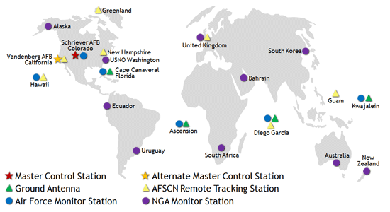
Control Segment
A reference network that continuously monitors the exact locations of the GPS satellite constellation. The locations of these ground stations are well known. To determine the locations of the satellites, it is the case of solving the GPS problem in reverse. These locations are then transmitted back to the satellites, such that this information can be re-transmitted back down to user GPS receivers.
The original GPS locations were in Hawaii (Eastern Pacific), Schriever U.S. Air Force Base in Colorado (North America), Ascension Island (South Atlantic), Diego Garcia (Indian Ocean), and Kwajalein (Western Pacific).
Over time, this original network has been augmented with additional stations.

The GPS operation “ground” control segment. Image from www.gps.gov (2018). https://www.gps.gov/systems/gps/control/map.png
One of the most important aspects of the control segment is keeping GPS time. The GPS system time is the synchronized time that all satellites share. Small differences can occur between GPS time and the satellite clock. Corrections can be handled either digitally (accounted for through the GPS signal) or physically (an actual change to the satellite clock).
User Segment
Similar to the Internet, GPS has become an essential part of the global information infrastructure. The free, open, and dependable nature of GPS has led to the development of hundreds of applications affecting every aspect of modern life. GPS technology is now in everything from cell phones and wristwatches to construction equipment, shipping containers, and ATM’s. (https://www.gps.gov/applications/)
Mobile Applications
In this course, we will be utilizing ESRI’s Collector for ArcGIS. The app is available for iOS, Android and Windows 10 devices. We will be installing them on the iPad 4 mini tablets.
Collector
Collector is one of several mobile apps provided by ESRI for ArcGIS. Collector requires you to have an ESRI account (this was created for you and consists of your Catawba username followed by “_catu”).
Before we begin using collector, we need to create a hosted editable feature service (feature layer), which can be done in ArcGIS Online. In the “Content” page, in the top left select “Create” –> “Feature Layer.”
Note: your account settings may not allow you to create a hosted feature layer, in which case, one will be created for you.
For feature layers, there are several templates that are provided by ESRI (e.g., “Field Notes”). Select the types of features (i.e., points, lines and/or polygons) you want to map. Specify the extents for your feature layer by zooming into or out of the map area. Give your feature layer a title.
Select your new feature layer to open its Overview page. In the top right, click the arrow next to “Open in Map Viewer” and select “Add to new map.”
You may edit your map settings (e.g., basemap, bookmarks, symbology). When you are done editing, click “Save” and give your new web map a title. You may share your web map with other users. All edits done to a shared web map will be accessible to all users.
Configuring Your Bad Elf GPS Receiver
On your iPad, in the maps view of Collector there is a symbol in the center of the menu bar at the top that looks like a box with an arrow pointed upwards. Click this symbol to open a menu. From the menu, select “Settings.” In the Settings window, under the “Location” header, click on “Provider” to open the “GPS Receivers” menu window. If your Bad Elf GNSS Surveyor has been successfully linked to your iPad and it is currently turned on, it will show up in the menu options. By default, the “Integrated Receiver” is selected, as indicated by the checkmark to the left of its name. Select the “Bad Elf, LLC” option, which should also include the receiver’s serial number. Click the “< Settings” in the top left of the menu to return to the “Settings.” Click “Done” in the top right of the menu to save your edits and close the menu.
Creating a Map for Collector
The following provides an example for creating a new file geodatabase, adding features and domains, publishing the feature class as a hosted service to ArcGIS Online, and adding it to a web map for Collector. While this example specifies values for a campus litter survey, the same procedure may be used for other field survey applications.
New Geodatabase
- Create a folder on your USB drive (e.g.,
F:\Project) - Start ArcGIS Pro
- Open a new blank project (
Preserve) - In Catalog, under Folders, find the project folder
Preserve - Right-click on
Preserveand selectNew --> File Geodatabase - Right-click the new geodatabase and rename it “fsjep_[YOURINITIALS]” (e.g.,
fsjep_twd.gdb) - Right-click on your geodatabase and select “Edit Metadata”
- Enter your geodatabase information:
- Title: Dr Davis Preserve Database
- Tags: Collector, GPS, Preserve, Catawba
- Summary: A file geodatabase for storing features for field surveys in the Fred Stanback, Jr. Ecological Preserve.
- Description: This file is a part of Catawba College’s ENV 3599 Intermediate GIS/Field GPS spring semester 2019 ecological preserve survey project. The goal of this project is to use GPS receivers to survey the preserve in order to create an informative map.
- Credits: Dr. Davis, Department of Environment & Sustainability, Catawba College, Salisbury, NC.
Add Feature Class
Create a new Feature Class in your geodatabase. You may create multiple feature classes within a single geodatabase.
- Right-click on the geodatabase in the Catalog and select
New --> Feature Class - Enter the information in the New Feature Class window
- Name:
manhole_survey - Alias:
Manholes - Feature Class Type:
Point - Geometry Properties: (leave options unchecked)
- Name:
- Click “Next”
- Fields
- Leave fields as they are for now
- Click “Next”
- Choose the feature’s spatial reference
- Projected Coordinate Systems
- State Plane
- NAD 1983 (US Feet)
- NAD 1983 StatePlane North Carolina FIPS 3200 (US Feet)
- NAD 1983 (US Feet)
- State Plane
- Projected Coordinate Systems
- Click “Next”
- Leave XY tolerance values as default
- Click “Next”
- Leave Resolution as default
- Click “Next”
- Leave database storage configuration as default
- Click “Finish”
For each feature class in your geodatabase, make certain you use the same coordinate system. Import the coordinate system from an existing layer to ensure it is the same across all your layers.
Add Additional Fields
Create new fields (attributes) for your feature class.
- Right-click “manhole_survey” feature class in the Catalog and select
Design-->Fields - At the bottom of the table, “Click here to add a new field”
- Enter a new field for the closest trail name
- Field Name:
TRAIL - Alias:
Trail - Data Type:
Text - Allow NULL values:
No(unchecked) - Domain: (leave blank)
- Default Value: (leave blank)
- Length:
50
- Field Name:
- Enter a new field for surveyor’s name (initials)
- Field Name:
SURVYR - Alias:
Surveyor - Data Type:
Text - Allow NULL values:
No(unchecked) - Domain: (leave blank)
- Default value: (your initials)
- Length:
4
- Field Name:
- Enter a new field for field notes
- Field Name:
NOTES - Alias:
Notes - Data Type:
Text - Allow NULL values:
Yes(checked) - Default value: (leave blank)
- Length:
255
- Field Name:
- Enter a new field for the timestamp
- Field Name:
DATETIME - Alias:
Date - Data Type:
Date - Allow NULL values:
No(unchecked) - Domain: (leave blank)
- Default Value: (leave blank)
- Field Name:
- Click “Save” in the Fields ribbon
Add GPS Receiver Fields
Create additional fields for recording the GPS receiver data1.
- Enter a new field for GPS receiver name
- Field Name:
ESRIGNSS_RECEIVER - Data Type:
StringorText - Alias:
Receiver Name - Allow NULL values:
Yes - Default value: (leave blank)
- Length:
50
- Field Name:
- Enter a new field for GPS receiver’s horizontal accuracy
- Field Name:
ESRIGNSS_H_RMS - Data Type:
Double - Alias:
Horizontal accuracy - Allow NULL values:
Yes - Default value: (leave blank)
- Field Name:
- Enter a new field for GPS latitude
- Field Name:
ESRIGNSS_LATITUDE - Data Type:
Double - Alias:
Latitude - Allow NULL values:
Yes - Default value: (leave blank)
- Field Name:
- Enter a new field for GPS longitude
- Field Name:
ESRIGNSS_LONGITUDE - Data Type:
Double - Alias:
Longitude - Allow NULL values:
Yes - Default value: (leave blank)
- Field Name:
- Enter a new field for GPS fix time
- Field Name:
ESRIGNSS_FIXDATETIME - Data Type:
Date - Alias:
Fix time - Allow NULL values:
Yes - Default value: (leave blank)
- Field Name:
- Click “Save”
Create Domains
Create and apply domains for your fields. These will be used in Collector for creating the selection boxes for attributes (i.e., saves you from having to type).
- In the Catalog, right-click on your geodatabase and select
Design-->Domains - In Domains ribbon, click on “New Domain”
- Create a domain for trail names
- Domain Name:
TrailName - Description:
Name of closest trail to manhole - Field Type:
Text - Domain Type:
Coded Value Domain - Split Policy:
Default Value - Merge Policy:
Default Value - Coded Values: as needed, for example:
- Code: Wurster
- Description: Wurster Trail
- Code: Pipeline
- Description: Pipeline Trail
- Code: BLoop
- Description: Birding Loop
- Code: Other
- Description: Other unnamed trail
- Code: None
- Description: Not located near to a trail
- Domain Name:
- Create a domain for surveyor initials
- Domain Name:
Surveyor - Description:
Surveyor initials - Field Type:
Text - Domain Type:
Coded Value Domain - Split Policy:
Default Value - Merge Policy:
Default Value - Coded Values: as needed, for example:
- Code: TWD
- Description: T. Davis
- Domain Name:
- Create a domain for the date and time
- Domain Name:
DateTime - Description:
Date and time of survey - Domain Type:
Range - Field Type:
Date - Split Policy:
Default Value - Merge Policy:
Default Value - Minimum value:
2019-01-01 00:00:00 - Maximum value:
2019-12-31 23:59:59
- Domain Name:
- Click “Apply”
- Click “OK”
Apply domains to fields and set default values.
- In the Catalog, right-click “manhole_survey” and select
Design-->Fields - Double-click the domain box for row
TRAIL- Under Field Properties, click in the box to the right of Domain and select “TrailName”
- Select
SURVYR- For Domain, select “Surveyor”
- For Default Value, type: [YOURINITIALS]
- Select
DATETIME- For Domain, select “DateTime”
Create attachments
Adding attachments to your feature class adds support for a variety of file types (e.g., photos). This is accomplished through a geoprocessing tool, “Enable Attachments.”
First, right-click on the feature class, “manhole_survey”, and select “Add to Current Map.”
Then go to geoprocessing tools: Data Management --> Attachments --> Enable Attachments.
Assign symbology
Create meaningful symbology for the various features in your map.
- Beginning with a new empty map, click on
File --> Add Data --> Add Data...(or click on the Add Data icon, ) and add the feature(s) from your geodatabase
 - In the Table of Contents, list by source
- Right-click your feature class (Litter) and select “Properties…”
- Click on Symbology tab
- Under Show, click Categories and select “Unique values”
- Under Value Field, select “Material”
- Click “Add All Values”
- Update Symbol and Label as desired
Note that 3D marker symbols are not currently supported in ArcGIS Online and therefore cannot be used with Collector.
Publish service
A personal file geodatabase can be published to ArcGIS Online as a hosted service for editing online, sharing with other users, and accessing with Collector.
- In ArcGIS Pro, from the Catalog, right-click the feature class you want to share and select “Add to Current Map”
- In the Contents pane, right-click the layer and select
Sharing-->Share As Web Layer - Provide the layer with a summary and tags (if you haven’t already).
- Select the web folder you wish to save it to.
- Choose who to share the layer with (e.g., Groups)
- Update the layer metadata, for example:
- Summary: A file geodatabase for storing features for field litter surveys.
- Tags: Collector, GPS, Litter, Catawba
- Description: This file is a part of Catawba College’s ENV 3599 Intermediate GIS/Field GPS spring semester 2018 litter survey project. The goal of this project is to use GPS receivers to survey campus litter and perform analyses using GIS geospatial tools.
- You may receive a warning that “Layer does not have a feature template.” You may ignore this warning as a default template will be created for you.
- Log into ArcGIS online to edit the layer settings, such as editing, updating, sync’ing, and downloading.
- Click on Sharing and select our group (i.e., ENV 3599)
- Click on Analyze at the top of the window and check to make certain no error messages appear (red x’s)
- Click Publish
Enable Edits, Sync and Export
In ArcGIS Online, find the newly create hosted feature class. Click on Settings in the top menu and scroll down until you see Feature Layer (hosted).
Check the boxes next to Enable editing and Enable Sync (you may also check the other two boxes for tracking feature creation and updates).
Scroll down to the bottom and check the box next to Export Data. This will allow you to download the hosted feature class as a shapefile in ArcGIS Pro.
Create web map
To use a hosted feature service with Collector, it must first be incorporated into a web map, which may be accomplished in ArcGIS Online.
- Open a web browser and go to https://arcgis.com
- Log in with your ESRI account details
- Click on Content
- Find your published Feature Layer (e.g., litter_survey_YOURINITIALS); note there should also be a Service Definition file with the same name
- Click the more details button next to your feature layer (i.e.,
...) and select “Add to a new map” - In the “Find address or place” search bar in the top right, type “Salisbury, NC” and click the suggestion option to zoom to Salisbury
- Zoom over Catawba College (this will be the default extents)
- Click Details at the top to open the Contents panel on the left
- Click on layer name (litter_survey_YOURINITIALS) to open the dropdown
- Click on the more options button (i.e.,
...) and select “Rename” - Rename your layer “Litter Survey”
- Zoom in over the Center for the Environment and click on “Bookmarks” and “Add Bookmark”
- Title the bookmark “Center for the Environment” and hit return
- Click the close box to close the bookmarks menu
- Zoom out so you see all of campus
- Click on Bookmarks and select “Center for the Environment” to zoom back to the center
- You can create other bookmarks if you wish; these will be available to you in Collector
- Here, you may also change the basemap style (currently set to Topographic)
- Click Edit in the menu at the top and select Manage at bottom of the panel on the left
- Under each material listing is a subheading; click the down arrow next to the subheading and select “Properties”
- Use the descriptions listed in Table 1 below to update the descriptions for each material
- Set the default values for the feature type template
- When your map is ready, click
Save --> Save As - Enter the information for your map
- Title: Litter Survey YOURINITIALS
- Tags: Collector, GPS, Litter, Catawba
- Summary: A web map for field litter surveying.
- Click “Save Map”
| Material | Property Description |
|---|---|
| Cloth | Clothing, upholstery, etc. |
| Foam | Styrofoam or polystyrene food and drink containers |
| Food | Apple cores, banana peels, sandwiches, etc. |
| Glass | Bottles, light bulbs, etc. |
| Metals | Soft drink cans, gum wrappers, etc. |
| Paper | Newspaper, cigarette butts, cardboard, napkins, etc. |
| Plastics | Spoons, straws, bags, etc. |
| Sensitives | Syringes, sharps, diapers, etc. |
| Wood | Popsicle sticks, coffee stirrers, etc. |
| Misc | Unclassified |
Share your map.
- Click on
Home --> Contentin the top left of the web map to return to your Content page - Next to your map, click the lock icon to open the Share window, check the box next to “ENV 3599” and click “OK” to share
Arcade
Arcade is a new secure and portable expression language with the goal of being able to run across all ArcGIS products (mobile, desktop and cloud)2.
The benefit of Arcade is its ability to create new derived attributes as on-the-fly calculations, rather than using the field calculator on a new field. This is handy for simple operations like changing the units of a field or calculating averages across fields without the overhead of storing the results in the database3.
Uses
- Ground truths
- Inspections
- Assessments
- Inventories
- Control points
- and others
Glossary
- A-GPS
- Assisted Global Positioning System (GPS)
- uses the range from GPS satellites, but receives the data (clock and satellite almanac) from a land-based cellular network to improve the time for GPS signal lock
- Apogee
- the proximal point in an object’s orbit; in the case of GPS, it is the point along the satellite’s orbit where it is closest to Earth
- ARNS
- Aeronautical Radio Navigation Signal
- a band of the radio spectrum allocated for aviation
- ASV
- Autonomous Surface Craft
- bands
- radio bands (or frequency bands) are used to break up the RF spectrum into nominal frequencies for transmitting information; these bands are then allocated to certain services
- C/A
- Course Acquisition (or Clear Access)
- a navigation signal code sent from GPS satellites
- Clock Phase
- the quantity that results when a flow or a rate is accumulated or summed
- Clock Rate
- the difference between two phase measurements divided by the duration of time that lapsed between taking the two measurements
- Constellation
- a system of satellites that work together to achieve a single purpose
- also called a “satellite swarm”
- DGPS
- Differential Global Positioning Systems
- EHF
- Extremely High Frequency
- RF band (30 GHz–300 GHz)
- EGNOS
- European Geostationary Navigation Overlay Service
- European SBAS
- Geodesy
- a scientific discipline dealing with the measurement and representation of the Earth, primarily: Earth’s shape, gravity field, and orientation in space
- it includes the quantification of properties of Earth’s surface and subsurface (e.g., crustal motion, ice sheets, glaciers, ocean tides and atmosphere)
- it utilizes GPS to continuously monitor changes in these properties
- GIS
- Geographic Information System
- visualization and analysis tool
- GLONASS
- transliteration: Globalnaya Navigazionnaya Sputnikovaya Sistema (Global Navigation Satellite System)
- Russia’s version of GPS
- GNSS
- Global Navigation Satellite System
- Special Topic: used in remote sensing (GNSS-R)
- GPS
- Global Positioning System
- data collection tool
- HF
- High Frequency
- RF band (3 MHz–30 MHz)
- L1
- Link 1
- GPS navigation signal frequency (1.57542 GHz)
- most commonly used GPS signal (supports 2–3 billion civilian receivers)
- L2
- Link 2
- GPS navigation signal frequency (1.2276 GHz)
- first used in 2005
- used by both civilian and military receivers
- provides a “backup” signal in the event L1 is unusable
- combined with L1, it helps cancel out the largest error source from the GPS signal
- LEO
- Low Earth Orbit
- this is where surveillance and spy satellites are located; it is closer to Earth than MEO, which allows for quality photographs of the surface to be taken
- LF
- Low Frequency
- RF band (30–300 kHz)
- Lock (or Fix)
- when a GPS receiver has a lock or fix, there are at least four satellites in good view in order to provide an accurate account of location and time
- MEO
- Mean Earth Orbit
- this is where the majority of GPS satellites are located; it is farther away than LEO, which provides about 1/3 of Earth’s surface in view of each satellite, reducing the total number of satellites required for global coverage
- MF
- Medium Frequency
- RF band (300–3,000 kHz)
- MSAS
- Multi-functional Satellite Augmentation System
- Japanese SBAS
- Multipath Error
- occurs when multiple instances of the same GPS signal are collected at a receiver due to the signal bouncing off obstructions (e.g., trees, buildings, other tall objects)
- NMEA
- National Marine Electronics Association
- develop specifications (format) for communicating GPS data
- NOAA
- National Oceanic and Atmospheric Administration
- Perigee
- the extreme point in an object’s orbit; in the case of GPS, it is the point along the satellite’s orbit where it is farthest from Earth
- Phase Cycle
- the periodic reset of a Clock Phase
- PRN
- Pseudo Random Number
- unique numeric look-up value assigned to satellites
- Pseudo Range
- distance calculated between a GPS receiver and a satellite with the presence of a phase error between the two clocks
- QNSS
- three frequencies patterned to complement GPS
- Range
- distance between GPS receiver and a satellite
- Rate
- the distance traveled over a given amount of time; a velocity
- RF
- Radio Frequency
- RNSS
- Radio Navigation Satellite System
- a band of the radio spectrum allocated for navigation satellites
- includes GPS L1 and L2 frequencies
- ROV
- Remotely Operated Vehicle
- PNT
- Position, Navigation and Timing
- services provided by GPS
- SBAS
- Satellite-Based Augmentation Systems
- complementary to GNSS; SBAS is a system of satellites and ground stations that provide GPS signal corrections to compensate GNSS accuracy, integrity, continuity and availability
- provides location accuracy within 3 meters
- see also EGNOS, MSAS and WAAS
- SHF
- Super High Frequency
- RF band (3 GHz–30 GHz)
- SV
- Space Vehicle
- another name for satellite
- TTFF
- Time To First Fix
- the time it takes for a GPS receiver takes to accurately compute your position and time using at least four satellites after it is powered on
- UHF
- Ultra High Frequency
- RF band (300 MHz–3,000 MHz)
- UNAVCO
- Originated as the University NAVSTAR Consortium in 1984; it is a non-profit university-governed consortium that facilitates geoscience research and education using geodesy
- USV
- Unmanned Surface Vehicle
- VHF
- Very High Frequency
- RF band (30 MHz–300 MHz)
- This band carried most early TV stations
- WAAS
- Wide Area Augmentation System
- North American SBAS
Appendix
Einstein’s Theory of Relativity
- Special Relativity
- Time flows differently according to the state of motion (i.e., events that are simultaneous for one observer may not be for another). This is represented by the famous equation: \(E = m c^2\), which shows that mass increases with speed. A conclusion from this work is that time slows down for objects in motion.
- General Relativity
- The Principle of Equivalence that states that acceleration and gravity are indistinguishable. Massive objects cause a distortion in space-time, which is felt as gravity. As a result, time does not pass at the same rate for everyone. Under more gravitational force, time travels slower.
Kepler’s Three Laws
- The Law of Ellipses
- All planets orbit the sun in ellipses with the Sun located at one focus of the ellipse.

Figure. Kepler’s Law of Ellipses (Ventrudo 2013). Copyright 2008–2018 Mintaka Publishing Inc.
- The Law of Equal Areas
- A line joining a planet and the Sun sweeps out equal areas during equal intervals of time. This is because as a planet gets closer to the Sun, it has less potential energy and more kinetic energy (i.e., planets move faster when they are closer to the Sun).

Figure. Kepler’s Law of Equal Areas (Ventrudo 2013). Copyright 2008–2018 Mintaka Publishing Inc.
- The Law of Harmonies
- The square of the orbital period, \(P\), of a planet is directly proportional to the cube of the semi-major axis of its orbit, \(a\) (i.e., planets move slower when they are farther from the sun and whatever influence makes planets go around the sun weakens with distance).
\(P^2 \propto a^3\)
Keplerian Elements
The orbits of the satellites are described using six Keplerian elements.

The Keplerian orbital parameters. Image modified from spaceflight.nasa.gov. Accessed 19 January 2018. https://spaceflight.nasa.gov/realdata/elements/graphs.html
where:
- \(a\) is the semi-major axis of the orbit ellipse
- \(e\) is the eccentricity of the ellipse
- \(i\) is the inclination angle; describes the pitch between the satellite’s orbital plane (hashed) and Earth’s equatorial plane (gray)
- \(\Omega\) is the angle of the right ascension of the ascending node; the angle between the vector connecting Earth’s center and the vernal equinox (along 0 degrees longitude at the Prime Meridian and 0 degrees latitude at the equator) and the vector connecting Earth’s center to the intersection of the equatorial and orbital planes
- \(\omega\) is the angle of the perigee of the satellite orbit
- \(\nu\) is the true anomaly; the angle describing the location of the satellite within its orbit with respect to the perigee
Newton’s Law of Gravity
Every point mass attracts every single other point mass by a force pointing along the line intersecting both points. The force is proportional to the product of the two masses and inversely proportional to the square of the distance between them (Newton 1687):
\(F = -\frac{G M m}{r^2}\)
where
- \(F\) is the force of attraction between two bodies
- \(M\) is the mass of one body
- \(m\) is mass of the second body
- \(r\) is the distance between two the bodies
- \(G\) is the gravitational constant (6.674 N m2/kg2)
Resources
Bad Elf GNSS Surveyor. Bad Elf. 2018. https://bad-elf.com/pages/be-gps-3300-detail
Do you know where you are? - The Global Positioning System. National Oceanic and Atmospheric Administration (NOAA). 2017. https://oceanservice.noaa.gov/education/tutorial_geodesy/geo09_gps.html
The Global Positioning System. Written by Peter H. Dana, Department of Geography, University of Texas at Austin. 1994. Provided by Ken Foote, The Geographer’s Craft, Department of Geography, University of Colorado at Boulder. 2015. https://www.colorado.edu/geography/gcraft/notes/gps/gps_f.html
GPS: An Introduction to Satellite Navigation (“GPS MOOC”). Stanford University. 2014. Available online: https://www.youtube.com/playlist?list=PLGvhNIiu1ubyEOJga50LJMzVXtbUq6CPo
GPS: The Global Positioning System. Maintained by the National Coordination Office for Space-Based Positioning, Navigation, and Timing. 2018. https://www.gps.gov/
GPS Basics. Written by Aaron Weiss (a1ronzo). Available online at SparkFun Electronics. Accessed 18 January 2018. https://learn.sparkfun.com/tutorials/gps-basics
GPS Tutorial. Trimble Inc. 2018. http://www.trimble.com/gps_tutorial/
Johannes Kepler: His Life, His Laws and Times. National Aeronautics and Space Administration (NASA). 2017. https://www.nasa.gov/kepler/education/johannes
National Geospatial-Intelligence Agency. https://www.nga.mil
References
Newton, Isaac. 1687. Philosophiae Naturalis Principia Mathematica. London: Royal Society of London.
Ventrudo, Brian. 2013. “Kepler’s Laws.” https://oneminuteastronomer.com/8626/keplers-laws/.